 Machine Learning Tutorials, Courses and Certifications
Hierarchical Clustering Analysis
Clustering is the most common form of unsupervised learning, a type of machine learning algorithm used to draw inferences from unlabeled data.
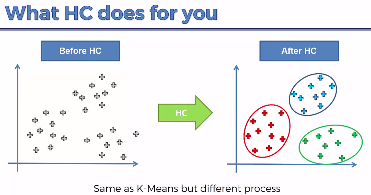
Hierarchical clustering, also known as hierarchical cluster analysis, is an algorithm that groups similar objects into groups called clusters. The endpoint is a set of clusters, where each cluster is distinct from each other cluster, and the objects within each cluster are broadly similar to each other.
Broadly speaking there are two ways of clustering data points based on the algorithmic structure and operation, namely agglomerative and divisive.
Hierarchical clustering algorithm is of two types:
i) Agglomerative Hierarchical clustering algorithm or AGNES (agglomerative nesting) and
ii) Divisive Hierarchical clustering algorithm or DIANA (divisive analysis).
- Agglomerative : An agglomerative approach begins with each observation in a distinct (singleton) cluster, and successively merges clusters together until a stopping criterion is satisfied.(Bottom to Top Approach)
- Divisive : A divisive method begins with all patterns in a single cluster and performs splitting until a stopping criterion is met.(Top to Bottom Approach)
Both this algorithm are exactly reverse of each other. So we will be covering Agglomerative Hierarchical clustering algorithm in detail.
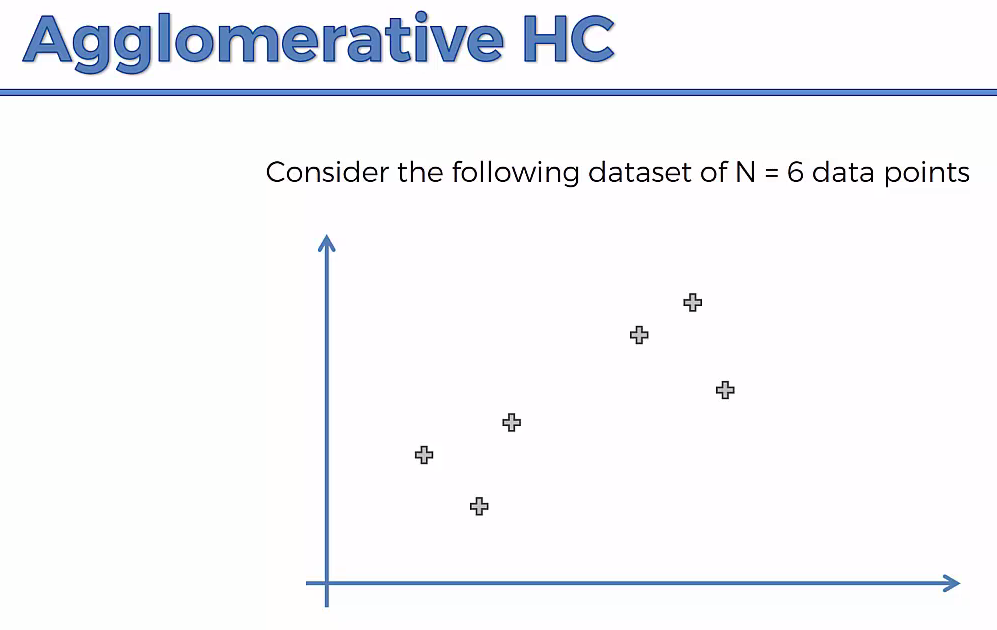
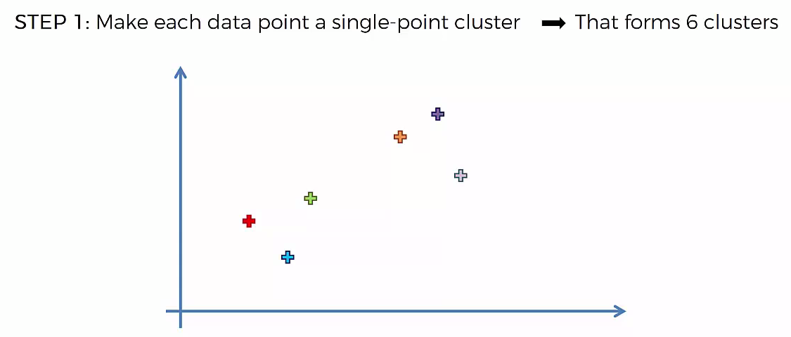
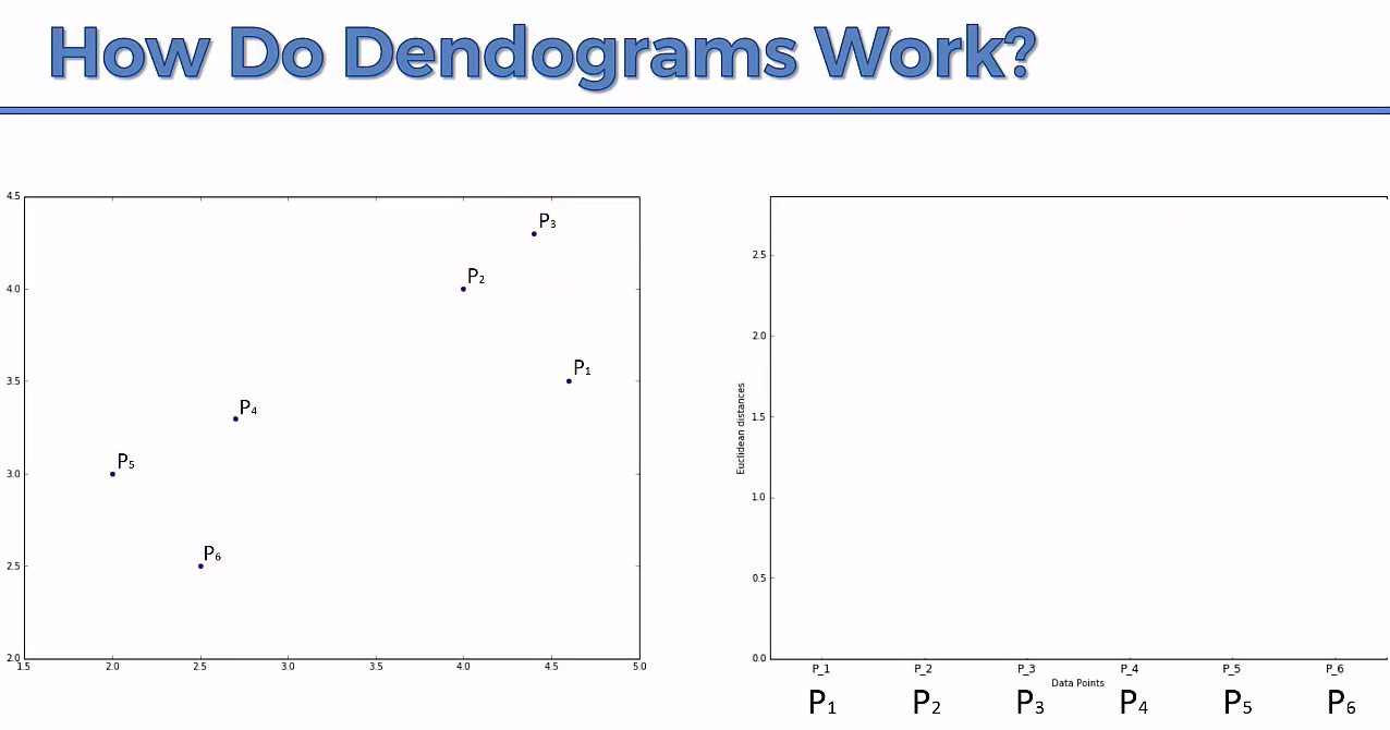
STEP 1: Make each data point a single-point cluster
- That forms N Cluster
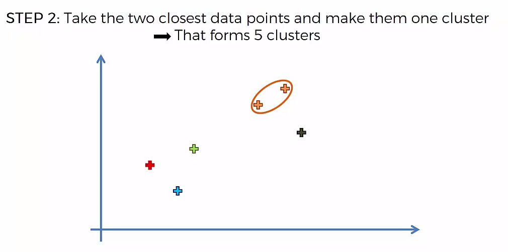
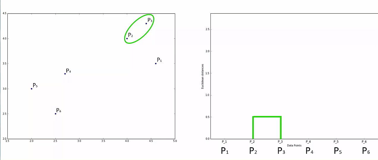
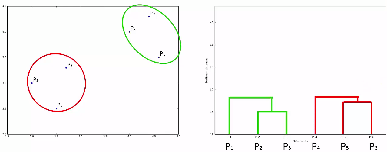
Step 2: Take the two closest data points and make them one cluster
- That forms N-1 clusters
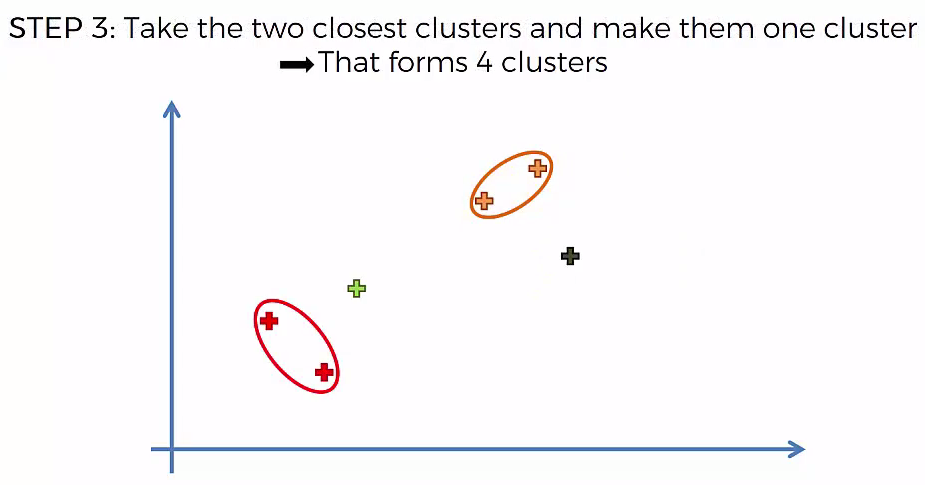
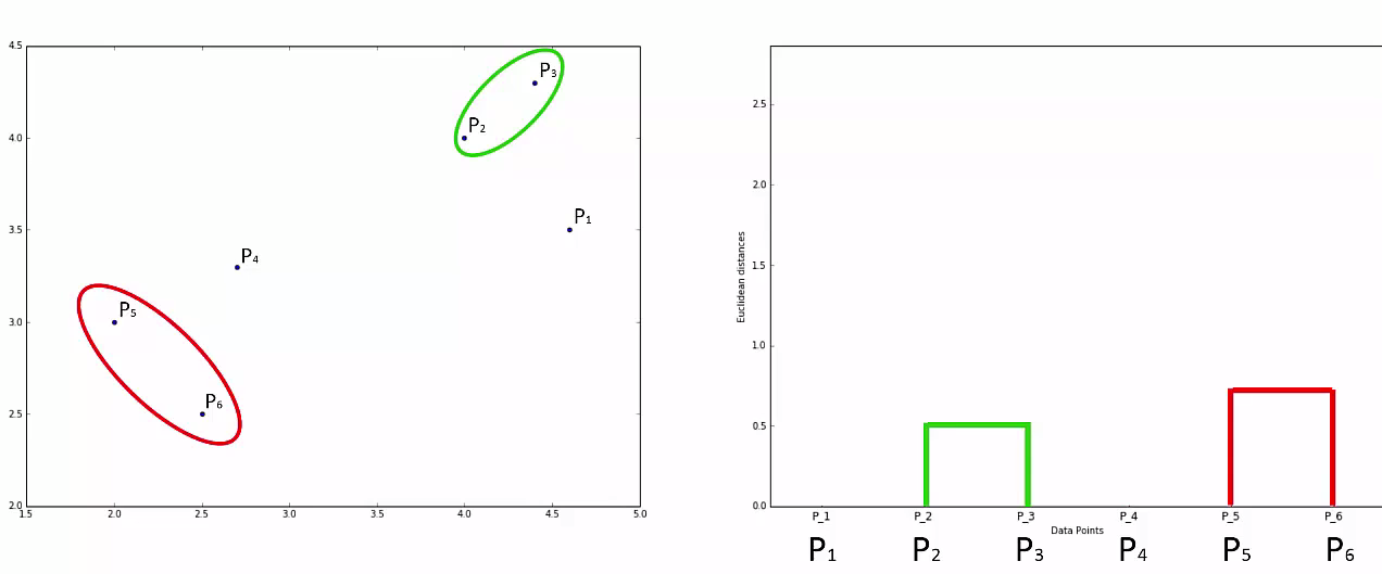
Step 3: Take the two closest clusters and make them one cluster
- That forms N-2 Cluster
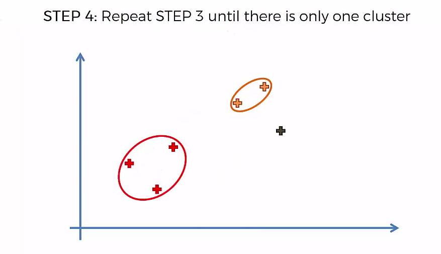
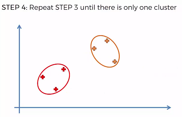
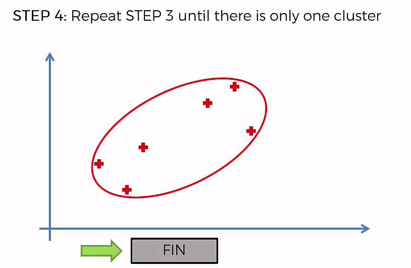
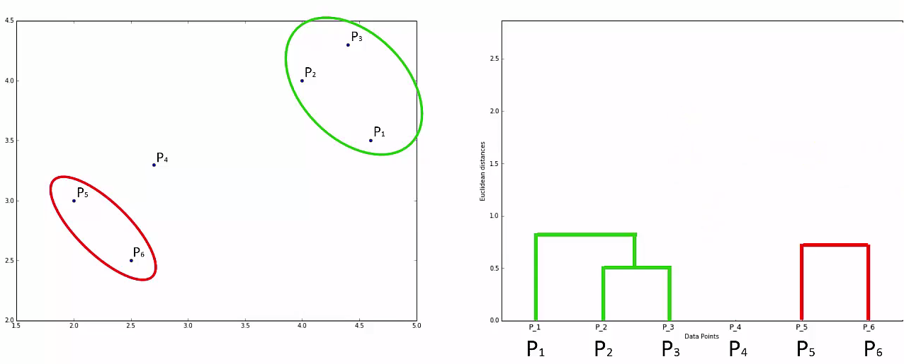
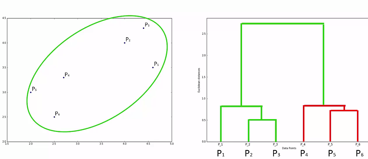
Step 4: Repear Step 3 until there is only one cluster
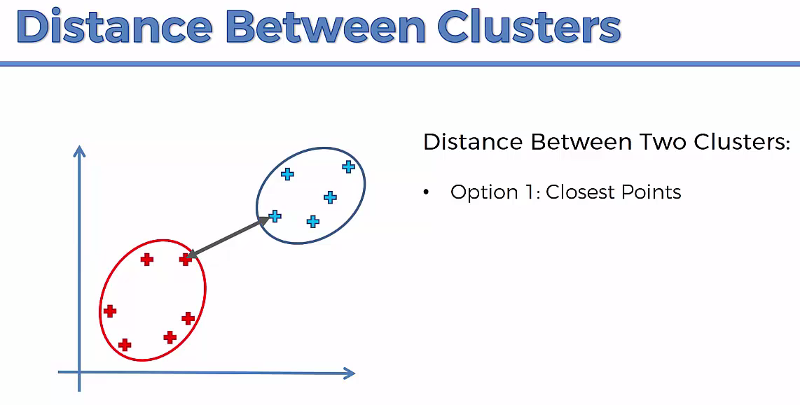
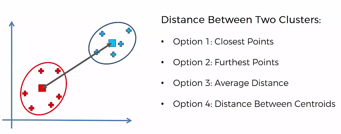
Agglomerative Hierarchical clustering -This algorithm works by grouping the data one by one on the basis of the nearest distance measure of all the pairwise distance between the data point. Again distance between the data point is recalculated but which distance to consider when the groups has been formed? For this there are many available methods. Some of them are:
1) Method of single linkage or nearest neighbour or Single-Nearest distance
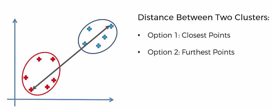
2) Method of complete linkage or farthest neighbour.
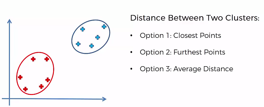
3) Method of between-group average linkage or average-average distance or average linkage.
4) centroid distance.
5) ward’s method – sum of squared euclidean distance is minimized. Ward’s method, or minimal increase of sum-of-squares (MISSQ), sometimes incorrectly called “minimum variance” method.
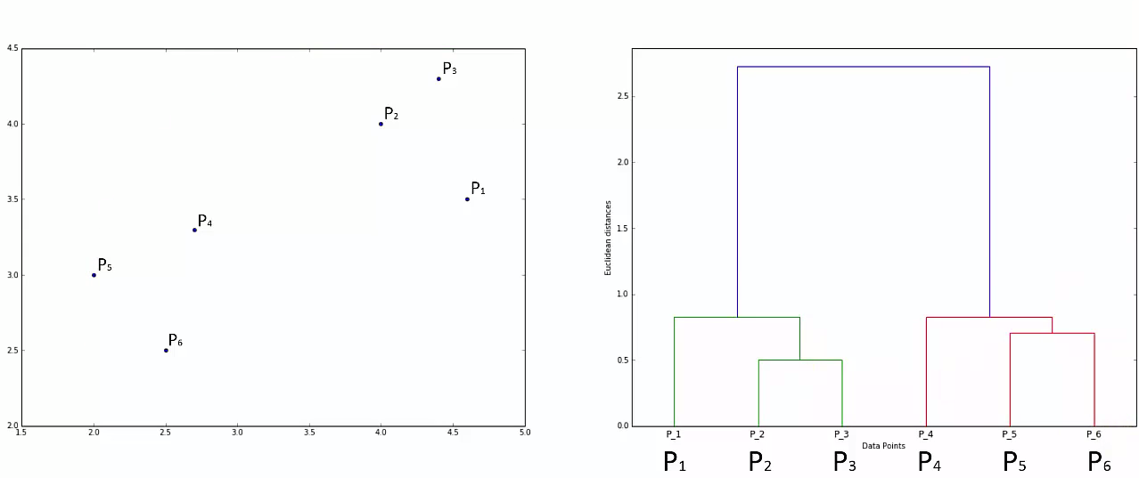
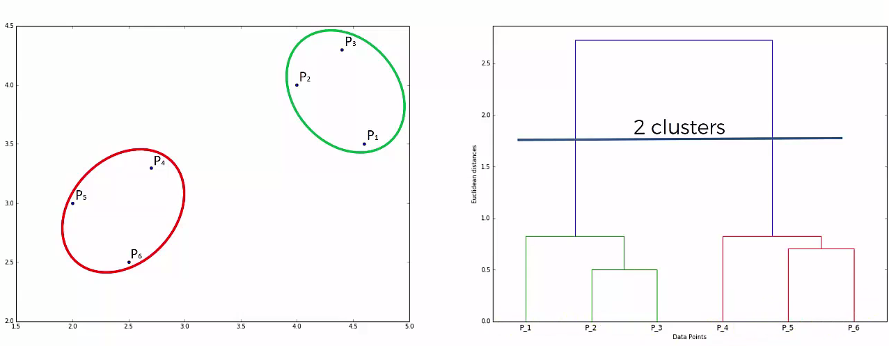
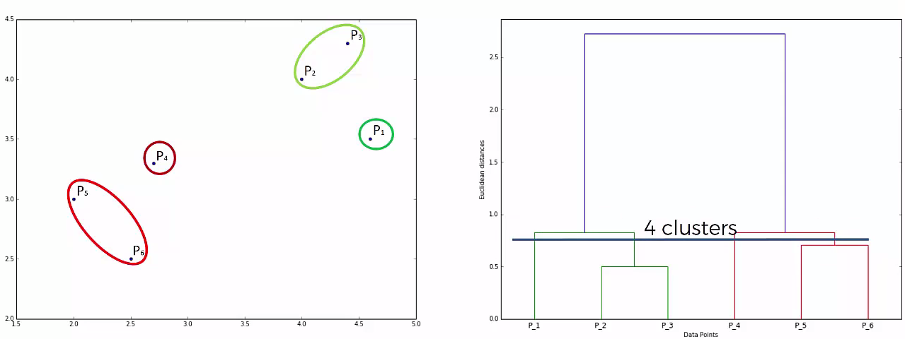
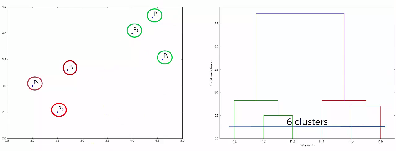
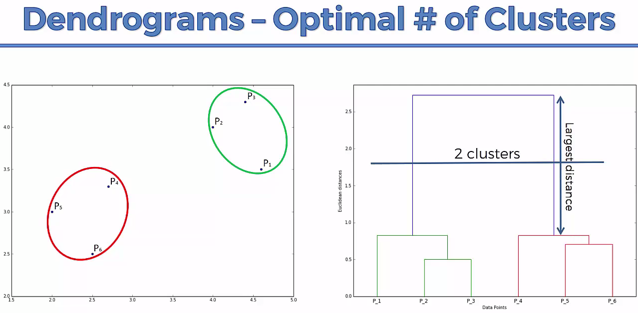
This way we go on grouping the data until one cluster is formed. Now on the basis of dendogram graph we can calculate how many number of clusters should be actually present.
Lets understand it practically
# Importing the libraries
import numpy as np
import matplotlib.pyplot as plt
import pandas as pd
# Importing the dataset
dataset = pd.read_csv('../datasets/Mall_Customers.csv')
X = dataset.iloc[:, [3, 4]].values
dataset
# Using the dendrogram to find the optimal number of clusters
import scipy.cluster.hierarchy as sch
dendrogram = sch.dendrogram(sch.linkage(X, method = 'ward'))
plt.title('Dendrogram')
plt.xlabel('Customers')
plt.ylabel('Euclidean distances')
plt.show()

# Fitting Hierarchical Clustering to the dataset
from sklearn.cluster import AgglomerativeClustering
hc = AgglomerativeClustering(n_clusters = 5, affinity = 'euclidean', linkage = 'ward')
y_hc = hc.fit_predict(X)
y_hc
# Visualising the clusters
plt.scatter(X[y_hc == 0, 0], X[y_hc == 0, 1], s = 100, c = 'red', label = 'Careful')
plt.scatter(X[y_hc == 1, 0], X[y_hc == 1, 1], s = 100, c = 'blue', label = 'Standard')
plt.scatter(X[y_hc == 2, 0], X[y_hc == 2, 1], s = 100, c = 'green', label = 'Target')
plt.scatter(X[y_hc == 3, 0], X[y_hc == 3, 1], s = 100, c = 'cyan', label = 'Careless')
plt.scatter(X[y_hc == 4, 0], X[y_hc == 4, 1], s = 100, c = 'magenta', label = 'Sensible')
plt.title('Clusters of customers')
plt.xlabel('Annual Income (k$)')
plt.ylabel('Spending Score (1-100)')
plt.legend()
plt.show()
